Numerical Methods: Newton Raphson Method Using Scilab

Because of the success of our previous post about the bisection method, we decided to also tackle the famous Newton Raphson Method in finding roots of an equation :)

But first lets ask wikipedia to define Newton Raphson:

Newton's method (also known as the Newton–Raphson method), named after Isaac Newton and Joseph Raphson, is a method for finding successively better approximations to the roots (or zeroes) of a real-valued function.

That did not tell us much, lets see the next paragraph:

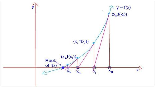
The Newton–Raphson method in one variable is implemented as follows:

Given a function ƒ defined over the reals x, and its derivativeƒ ', we begin with a first guess x₀ for a root of the function f. Provided the function satisfies all the assumptions made in the derivation of the formula, a better approximation x₁ is

Now thats better, the equation above uses the derivative of the function to determine the next estimate of the root. The way I remember Newton's method is that it takes the slope on the specific point (say X0) then using the value to estimate the next X and this goes on until the error is acceptable. Like what is shown in the picture below the value of X gradually diverges to the root!

Source:tutorvista

Newton's method is a lot faster compared to the bisection and it only takes in a single guess (one less thing to worry about). The Scilab code below uses the plotThatThing function that will again show the graph of the function and the location of the roots in an interval.

The Scilab Code:

Load this first before using

//this will plot the given function/expression in the given interval
function plotThatThing(theFunction, xLeft, xRight, theStepSize)
    x = xLeft : theStepSize : xRight;
    y = evstr(theFunction);
    plot(x, y, x, 0); 
endfunction

Now the code below is the actual Newton's Method in Scilab, it will take in two strings theFunction and theFunctionPrime and two values, the first is the guess and the second is the acceptable error. The guess can either be on the left or the right of the root it will still go to the root (not always but it might hehe).

//This function will use plotThatThing which is declareed on a different .sci file please load it first
function [root]=MyOwnNewtonRhapson(theFunction,theFunctionPrime, theGuess, acceptableErrorInPercent)

    //plot the function to get a look on how should it look
    plotThatThing(theFunction, theGuess - 100, theGuess + 100, 0.001);
    root = 0;
    relativePercentError = 100;
    numberOfIterations = 0;

    xsub0 = theGuess;

    x = xsub0;

    while  numberOfIterations < 100

        xPlusOne = x - (evstr(theFunction)/evstr(theFunctionPrime));

        x = xPlusOne;

        relativePercentError = evstr(theFunction) * 100;

        numberOfIterations = numberOfIterations + 1;     
    end

    root = x;

 endfunction

Advantges of Newton-Raphson Method:

Its fast!

Takes only one guess (one less thing to worry about compared to the bisection method covered before)

Pitfalls of Newton-Raphson Method:

It does not always converge - it might not be able to see the root and just go back and forth the root specially if the roots are close to each other (this one is based on experience this should not be taken as a generalization)